A two-wheel self-balancing robot
As written on my home page, I am currently studying to get a Bachelor Degree in Computer & Systems Engineering. Turns out that includes a ton of control theory and I’m enjoying it a lot. For my Automation exam, we had the option to have part of the exam evaluated on a project we realized. The lectures were divided in two separate modules, one about general theory and analysis for industrial automation, PID Controllers, Petri Nets, Finite State Machines and the like, and the other about Real-Time Scheduling of tasks. In the second part we also touched briefly on microcontrollers and embedded computing and we could choose to realize a project using those, which would count as part of the exam instead of a dedicated written test.
I obviously chose the project and, since I had been thinking and experimenting for a while, I decided to build a two-wheel self-balancing robot. I went a bit off track, but the professor was okay with it.
What follows is mostly an english translation of the essay I produced for the presentation of the project for the exam, with some added humour and errors I made which wouldn’t cut it during a presentation for an exam. It’s also probably the first time that I feature much math in a blog post and in general this could be the most complex project I’ve posted about yet. This is also the only page on my blog (yet) that requires javascript. I prefer to keep this site static, but this time javascript is needed to display LaTex equations. Finally, I want to add that this robot is kinda crap, and I built a v2 that fixes the errors I made in the v1 and adds some much needed features, but most of the concepts used in the v2 come directly from this one so it’s still very important to learn. The v2 will be featured in a future post.
I wanted to do things properly and apply all the knowledge I had gained in university thus far. If you search for “self balacing robot” on the internet, most of the results are about arduino projects that tell you to “just use a PID controller” and give you some random values for $K_P, K_I$ and $K_D$ without actually explaining how they got there, nor why a PID Controller is fit for the job in the first place. While using a PID controller is, in fact, not wrong at all (though it depends on what you want to actually achieve. In my case it was more than enough. I’ll go more in depth about it later) and neither is tuning it empirically, most of these projects directly use the output of the PID controller as the PWM value to feed to the motor drivers instead of some actual physical variable like motor torque. In general, they discard the physics and the maths behind such a robot, which are always important to look into.
Given this, I want this blog post to serve not only as the story of the development of a project of mine, but also as a kinda formal tutorial on designing such a robot, since there aren’t many around outside research papers. So I’ll try to keep things relatively simple and make them more complex when needed. I’ll assume whoever is reading this has a basic understanding of general physics, calculus and control theory, because of course I can’t explain them in the span of a blog post (and it’s already going to be a lengthy one). I hope the story of my struggles to bridge theory as explained in university and practice as needed by a pratical project will be useful to someone else that finds themselves in such a position.
So since the general internet was useless and I needed some guidance, I started looking into research papers that had realized such robots and I found a few interesting ones (some others were crappier but who am I to judge in the end, but a very desperate student). It helped that I already knew what I was looking for and the process I wanted to follow, because I already done some of this in different exams during the last two years in uni.
Write a (simplified, if needed) mathematical model of the robot. The robot dynamics is a physical process and we can derive a mathematical model of it. Since it’s a dynamic process (meaning there are forces and accelerations present), I expect it to be described by second order ordinary differential equations (ODE).
From the ODEs, derive a state space and/or a transfer function model, so that I can use the control engineering methods I already know.
Design a controller for the process since, spoiler, I already know it is unstable on its own (how? read further)
Simulate process and controller in Matlab/Simulink. This is needed to tune the controller parameters and to test I did not make huge mistakes before I actually buy the parts and build this robot (spoiler: I did make a huge error in the simulations that I discovered only after buying the wrong parts)
Actually build this robot. This will probably require a slight re-tuning of the parameters, but since we are smart and already studied the mathematical model and made simulations we should be pretty close to the correct ones, except for imprecisions of physical parameters like inertia, and if we are not we should be able to know what to change and test again on the real robot.
During this whole process I read a lot of research papers and got a little bit of useful informations and learnt new methods from each of them. When possible (i.e. there are free/not paywalled/not requiring an instutional account version available) they are linked throughout this post. When not possible, they are all listed at the end of this page and in my original essay.
1. Mathematical model
When it comes to derive a mathematical (specifically dynamic, in this case) model of a physical process, there’s two main paths you can chose: the first is using Newton’s second law of motion both for linear motion and rotations, and the second it to write the Lagrange’s equations.
But even before this, we have to understand the process we are dealing with. Let’s also make some assumptions to make our life easier: let’s say that we do not have two wheels, but a single one controlled by a single motor. No two motors are exactly the same, but this is a safe enough assumption to make if we use two motors with no extreme visible differences. This means that the robot cannot rotate along the z axis, but we will look into this in a future post. Let’s also assume no-slip movement, meaning the wheels always have friction with the terrain, and that the wheels are always touching the terrain, meaning the robot cannot bounce up and down.
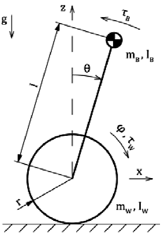
In general, problems like this belong to the family of inverted pendulums (eventually, on a cart). No, not the Yu-Gi-Oh kind of pendulums, the timekeeping device type.
Some simple examples of inverted pendulums? Try to balance a pole on your hand. The pole is the inverted pendulum, you are the controller trying to keep it balanced. Same applies to a person on a monocycle or an hover board: the person is the pendulum, the vehicle below is the cart. Even a person itself is an inverted pendulum: you are constantly using your muscles to keep yourself upright. The analogy becomes even better when you fall so out of balance that you need to walk forward or backwards to regain balance. That’s exactly what our robot will do: move forward or backwards to keep balance. Our robot is therefore nothing more than a glorified inverted pendulum on a cart, where the body of the robot itself is the pendulum and the wheels are the cart. This is why I already knew the robot would need a controller to stay upright.
By observing the scheme above (and also, by just thinking about it), we can observe that under the assumption we made the robot has two degrees of freedom, meaning two “movements” indepedent of each other: it can translate along the x axis and it can rotate along the y axis. We expect to have as many equations in our system as there are degrees of freedom. This is reflected quite well by using Lagrange’s equations, which is what I used to derive my model. This is only a personal preference, I honestly find them much more easier to manipulate compared to using Newton’s second law. I did the calculations on my own, but I also found this paper and followed along to check for errors. Plenty of other papers use newton’s, for example this one (which is cited by just about everyone), which however also considers the additional degree of freedom of rotation around the Z axis given by the presence of two independently actuated motors.
Lastly, the torque of the motors will be the input to the system that we have control over.
By following the first paper up until to step 2.14 we obtain this set of equations. Check the paper for the exact derivation, it’s pointless for me to write in again here:
\begin{equation} \begin{cases} (I_b+m_bl^2)\ddot{\theta} + m_bl\ddot{x}\cos\theta - m_bgl\sin\theta = -(\tau_r + \tau_l) \\ (m_b + \frac{2I_w}{r^2} + 2m_w) \ddot{x} + m_bl\cos\theta\ddot{\theta} - m_bl\sin\theta\dot{\theta}^2 = \frac{\tau_r + \tau_l}{r} - 2b_w\frac{\dot{x}}{r^2} \end{cases} \end{equation}
Which is, if I may, a rather ugly non-linear system. There are trigonometric functions, some variables are to the second power, sometimes variables are multiplied by their own derivatives. Sometimes the derivatives are to the second power. Oh, also I know nothing of non-linear systems. Luckily we can linearize this system around an equilibrium point, meaning that we fix a point around which the non-linear behaviour can be approximated with a linear one. If you think about an inverted pendulum, you’ll realize that they indeed have an equilibrium: that’s when they are perfectly vertical. It’s also a so-called static equilibrium, meaning than any infinitesimal disturbance will bring the system out of equilibrium and into instability.
Anyway, by noticing that around the equilibrium point $\theta = 0$ we have $\theta \ll 1\ rad$, meaning $\sin\theta \approx \theta$ and $\cos\theta \approx 1$ and ${\dot\theta}^2 \approx 0$
By substitution we obtain a linear model for our process, and we like this because control theory for linear systems is well know and estabilished and we can use all the tools and knowledge we already have.
\begin{equation} \begin{cases} (I_b+m_bl^2)\ddot{\theta} + m_bl\ddot{x} - m_bgl\theta = -(\tau_r + \tau_l) \\ (m_b + \frac{2I_w}{r^2} + 2m_w) \ddot{x} + m_bl\ddot{\theta} = \frac{\tau_r + \tau_l}{r} - 2b_w\frac{\dot{x}}{r^2} \end{cases} \end{equation}
We have reached our first goal: this is a mathematical model of the robot, expressed by Ordinary Differential Equations. As we expected, a system of two equations of the second order (meaning there the second derivates are present) and therefore dynamic.
2. Transfer function model
From here, what we are really interested in is a transfer function in the Laplace/frequency domain, based on which we can design a controller to keep the system around its equilibrium point. If I replace the values for my robot
| Name | Parameter | Value |
|---|---|---|
| $b$ | coefficient of friction of the wheels | 0.001 |
| $g$ | acceleration of gravity | 9.81 m/s^2 |
| $r$ | radius of wheels | 0.032 m |
| $l$ | distance from wheels to center of mass | 0.035 m |
| $ M_{body} $ | Mass of the robot, wheels excluded | 0.232 kg |
| $M_{wheel}$ | Mass of a single wheel | 0.012 kg |
| $I_{body}$ | inertia of the robot, wheels excluded | 9.4733e-05 kg m^2 |
| $I_{wheel}$ | inertia of a single wheel | 1.2288e-05 kg m^2 |
I get the following transfer function, expressed in the zero-pole-k form.
$$ \begin{equation} P(s) = \frac{\Theta(s)}{\tau(s)} = -13288 \frac{s+183}{ (s+921.7) (s+14.31) (s-14.68)} \end{equation} $$
How did I get those values? I eyeballed them! I knew which components and materials I wanted to use, so I designed a quick and rough structure in OnShape. OnShape also estimates the weight of some materials and I used those values to do an initial run of simulations. If I got those values wrong, and I probably have, I can always run more simulations until they are as close as possible to the real robot. In this case it’s always good to overestimate parameters like weight and inertia, which at most would cause me to buy oversized actuators than needed. When it comes to actuators, overspec’ing them a little does no harm; on the other hand, if I underspec’ed my parameters and thus the capabilities of my actuators I might end up getting actuators that are unfit for the job. You also don’t need to make an exact CAD model of the robot. Just eyeball the parameters with the components you intend to use and run more simulations to see how different parameters such as mass and wheel radii affect your model. You think your robot will weight 500 grams? Check what happens if it weighted a kilogram. Try to reduce or increase the radius of the wheels, does that require more or less torque from the motors? Are the results aligned with what you would expect from your physics knowledge? No? Check if you made any errors. It’s important to run these experiments early on to catch stupid errors. And always always check that you’re using the correct units of measure. Don’t be like me: I run most of my simulations in kilograms instead of grams and ended up buying motors way too oversized for what I needed. So oversized, in fact, that can exert a whopping 6 Nm of torque (the robot actually needs way less than 1 Nm) but could only turn at a measly 22 RPM (while the robot required more than 100).
We can observe the transfer function has two poles with a negative real part. Those are stable poles, because eventually they will converge to 0. The remaining pole has a positive real part and will eventually diverge to infinity. The presence of this single unstable pole makes our whole robot unstable, thus needing a controller to keep it upright.
Also, by deciding that our input-output transfer function is $F(s)= \frac{\Theta(s)}{\tau(s)}$ we are stating that the input of our system if the torque $\tau$ which will be applied by our motors and the output we are interested in is the pitch angle $\Theta$. Also, since we assumed to have only one motor for the sake of simplicity, we can safely say that the total torque $\tau$ is the sum of the torques applied by each motor, $\tau_{r}$ and $\tau_{l}$
3. Controller
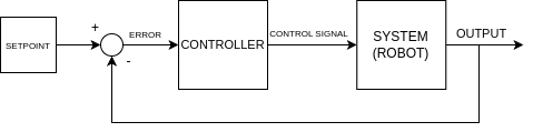
Now that we have a transfer function in the Laplace domain and we estabilished that we need a controller to keep the system (i.e. robot) into stability (i.e. upright) let’s try to design one.
We will use a classical feedback loop. We will measure the output of the system, which we decided to be the pitch angle $\theta$, compare it with a reference angle which is our desidered pitch angle, compute the error and feed it into the controller. The controller will do its magic and output a torque, which is the torque the motors must apply in order to keep the robot upright.
For the controller, I decided to use a PID Controller, because they are the most used controllers in industrial automation and also because they were a central part of the lectures for the exam for which I am making this robot. Basically they were the only thing keeping this project on track (evitare di andare fuori traccia).
Now, a PID controller is a linear system, and as such it makes sense to use it to control linear systems. Yet our robot is a non-linear system. But remember we are operating around an equilibrium point, when the non-linear behaviour can be approximated with a linear one. Using a PID Controller is therefore a correct choice, as long as the assumptions under which we made the linear approximation stay valid.
The transfer function of a PID controller in Laplace is:
$$ \begin{equation} C(s) = K_P + \frac{K_I}{s} + s K_D \end{equation} $$
A PID Controller takes three independent actions:
One proportional to the error itself (gain $K_P$)
This is the most intuitive action: more error means more action to correct it. If $K_P$ is set too low the response of the system will be way too slow. If $K_P$ is set too high we might saturate our actuators and set the system into oscillation.
One proportional to the integral of the error (gain $K_I$)
An integral action is used to “keep track of the history of the error”. Basically, if we have been off from the reference for some time we need to take a stronger control action. For a self-balancing robot, this value if usually the highest.
One proportional to the derivate of the error (gain $K_D$)
This is needed to avoid oscillations, or at least to drastically reduce their entity.
The derivative of the error is its rate of change. Basically, we try to look into the future to predict how the variable is going to change. But this would break causality and punch a hole into the fabric of reality, destroying the universe itself. I’m sure that’s a Doctor Who reference. Since we are not in Doctor Who and we cannot take a peek into the future, we say that a PID Controller with such an action is ideal. In practice, we would need another pole far away from the others which sets the pass band of the controller, inside which the derivate action can be taken. Also in practice, since we are going to implement the PID Controller digitally on a microcontroller, we can ignore this last bit and simply calculate the derivative as the difference of the current value of the error from the last one, then divide by the time that has passed. More on this later.
But how do we set this parameters?
Well, trial and error is a solution. It’s called the manual method and goes like this:
- Increase $K_P$ until you bring the system into oscillation, then set $K_P$ to half of that value. Note that if the system does not already have a pole in s=0, a proportional control alone cannot bring the error down to 0 at steady state.
- To bring the error to 0 at steady state we need an integral factor. Increase $K_I$ until the error converges to 0 as fast as you need. Mind you, if $K_I$ is too high you can saturate the actuators and therefore bring the system into oscillation or even instability. Also, with too high value of $K_I$ you start having wind-up problems.
- At this point there’s probably still some oscillations before the error converges to 0 and the steady state is reached. Try to increase $K_D$ in little steps to reduce the entity of these oscillations. Mind that a too high value of $K_D$ can cause “nervous” control (when the actuators quickly change direction and amplitude) and even instability if the actuators are brought into saturation.
We can also study the system analitically and get some conditions and constraints over the three parameters, then experiment with those. Alert: this next part requires a little bit of knowledge of control theory.
We can rewrite the PID controller as:
$$ \begin{equation} C(s) = \frac{s^2 K_D + s K_P + K_I}{s} = K_D \frac{s^2 + s \frac{K_P}{K_D} + \frac{K_I}{K_D}}{s} \end{equation} $$
The system can also be rewritten for generic values of poles, zeroes and gain. This is convenient to us, because changing some of the physical parameters of the robot, like mass or radii of wheels, will change the numerical value of the poles, the zeroes and the gain. It’s much better to do the calculations once with an algebraic method instead of repeating them with numbers each time we change a single parameter.
$$ \begin{equation} P(s) = K\frac{s+z_1}{(s+p_1)(s+p_2)(s-p_3)} \text{ with } K, z_1, p_1, p_2, p_3 \gt 0 \end{equation} $$
The numerator of the PID controller is a quadratic polynomial, so we can choose the parameters to have two distinct real roots. To obtain some constraints on the values of the parameters, we can simplify the two zeroes of the controller with the two stables poles of the process. This is a rather standard procedure to obtain constraints for the values of parameters and to ensure that the whole process (controller + system) has minimum dimension (meaning the least amount of poles possible). By using zeroes in the controller to cancel out poles in the process we make the corresponding eigenvalues observable but not controlable. We don’t really care, since we know they converge to 0 anyway.
By using $ s^2 + s \frac{K_P}{K_D} + \frac{K_I}{K_D} $ in the controller to cancel $p_1$ and $p_2$ out we obtain some conditions on the parameters.
\begin{equation} \begin{cases} \frac{K_P}{K_D} = p_1 + p_2 \\ \frac{K_I}{K_D} = p_1 \cdot p_2 \end{cases} \end{equation}
The open-loop process is therefore
$$ \begin{equation} F(s) = C(s) \cdot P(s) = KK_D \frac{s+z_1}{s(s-p_3)} \end{equation} $$
And the closed-loop process is:
$$ \begin{equation} W(s) = \frac{F(s)}{1 + F(s)} = \frac{N_F(s)}{N_F(s) + D_F(s)} = KK_D\frac{s+z_1}{s(s-p_3)+KK_D(s+z_1)} \end{equation} $$
And by applying Routh’s criterion to $W(s)$ we obtain the final condition on KD
$$ \begin{equation} K_D \lt -\frac{p_3}{K} \end{equation} $$
From here, we can test different combinations of parameters, by just setting $K_D$ and using the corresponding $K_P$ and $K_I$ we get from the analytical relationships we found. We will do all of this in a simulation in Matlab and Simulink.
4. Simulation in Matlab/Simulink
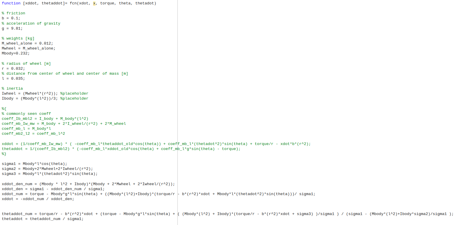
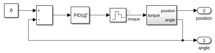
I used Simulink to create a block diagram of my robot and simulate it. While the controller is designed on the linear approximation of the system, it’s good to do simulations on the original, non-linear system, to be closer to reality. I implemented the system as a “Matlab function” block in Simulink, calculating $\ddot{\theta}$ and $\ddot{x}$ as we calculated in step #1. To avoid algebraic loops, I have written another script in Matlab that rearranges the equations to obtain one that only contains $\ddot\theta$ and another that only contains $\ddot{x}$. Here’s the script, from this project’s repo. In hindsight, I could have just used unit-delays to avoid algebraic loops
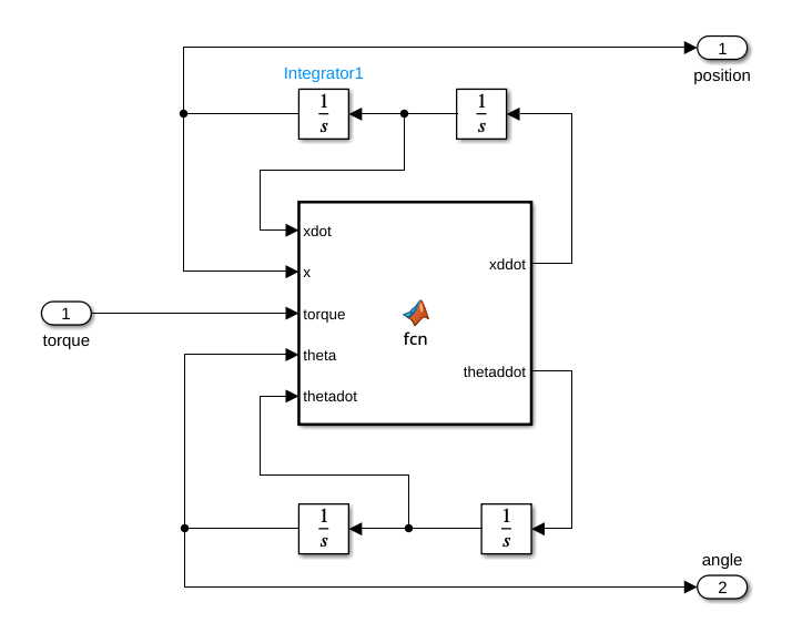
Another script takes in the linearized equations, replaces the numerical values for mass, radius, inertia, etc, calculates the open-loop transfer function, extracts poles, zeroes and gain and the prints the numerical constraints for the PID parameters. It also takes as input a value of $K_D$, calculates the corresponding $K_P$ and $K_I$ and then launches a simulation of the non-linear system controlled by a PID controller with the calculated values for $K_P$, $K_I$ and $K_D$
This process helps me tune the PID parameters with some guidance, so I don’t just have to trow stuff at the wall and see what sticks. As I explained earlier, I also use this process to study how different physical parameters affect the robot, in particular how much torque is required and thus which motors to buy, because remember, we have to buy actuators (motors in our case) for when we’re going to build the robot. We absolutely cannot go blind on this. If we had a bit of experience with mechanics, which I unfortunately lack, we could probably dimension the motors by eye. We could also overestimate the torque our motors need to output by a lot, but that would probably require bigger and more expensive motors and let’s say I’m on a budget here (also usually, the higher the torque the lower the RPMs, and we also need to make sure our motors can spin as fast as we need)
Since the PID is gonna be actually implemented on a microcontroller, we need to simulate a discrete time PID Controller, meaning that the output will be evaluated at fixed timesteps. Discrete time systems are a bit different to continous time systems but I won’t get deep into the differences in this post. The problem at this point is that while the microcontroller (and therefore the PID controller) are discrete-time systems, our robot itself is still a continous time system. That’s why we use a Zero-Order Hold to hold (as in mantain at the same value) the output of the system between a timestep and the next, otherwhise we would just have an impulse signal each time step, and zeroes in between.
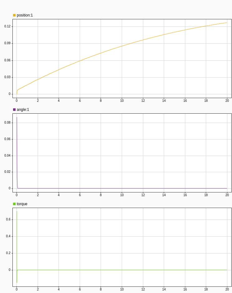
As I keep saying, we are using the simulations to study the behaviour system, in particular how much torque we need to apply using the motors to keep the system stable. But the actuators we’re gonna buy are far from ideal, and have some limits: they cannot apply an infinitely high torque. In fact, all motors have a max torque they can exert, after which they just stall and do not turn anymore. The datasheet of the motors you’re gonna buy should express this value as stall torque or something similar, and obviously you want to buy motors that have a stall torque higher than the max torque the controller will need to apply.
While we’re at it, we can also put some saturation limits on the PID Controller. Put simply, we are clamping (or constraining, if you will) the possible torque to be output to never go above a maximum or below a minimum. This way we can study what happens to our system when the actuators are in saturation, i.e. the motors are stalling and cannot exert more torque.
Based on some extensive testing I can say my robot should work if the motors can exert at max 0.65 Newton-meters of torque. But remember, for the assumptions we made this corresponds to the combined torque of both motors, so each motor needs only to be able to exert 0.33 Nm of torque. I settled for some Hitech HS-322D that I had laying around. From the datasheet, they have a stall torque of 0.37Nm. Here I made an error by not giving myself enough leeway with the motors: I should have bought new motors that had a slightly higher stall torque. The error came to bite me later. In fairness, those motors where only a backup solution, as a first I got my measurment units wrong, and performed all the simulations with all the masses expressed in kilograms instead of grams. This meant I simulated a 900kg robot barely 5cm tall. I wonder if that is at the limit to be considered a black hole. I ended up buying motors that could exert 6Nm of torque, but could only spin at 22rpm at max, which wasn’t barely fast enough for this robot. (Bonus: to check rpm, convert the linear velocity in the robot subsystem into rpm and plot those, then buy motors that can spin fast enough)
5. Building it
As I said in paragraph 2, I used OnShape to design the chassis of the robot. I daily drive Linux, and for a long time I used Fusion 360 in a Windows VM with a virtual GPU passed through. That setup was way too convoluted and unstable, so I decided to drop it and give OnShape a try. I’m yet to find the courage to dip my toes into FreeCAD.
Now, since I have access to a pretty nice FabLab. I decided to design the chassis of the robot to be laser cut, and only have a couple parts holding the electronics 3d printed. the 3d-printed parts are small and fast to print, and laser cutting is way faster than 3d-printing, which in all saved some significant manufacturing time, only at the cost of a little care when designing the parts.
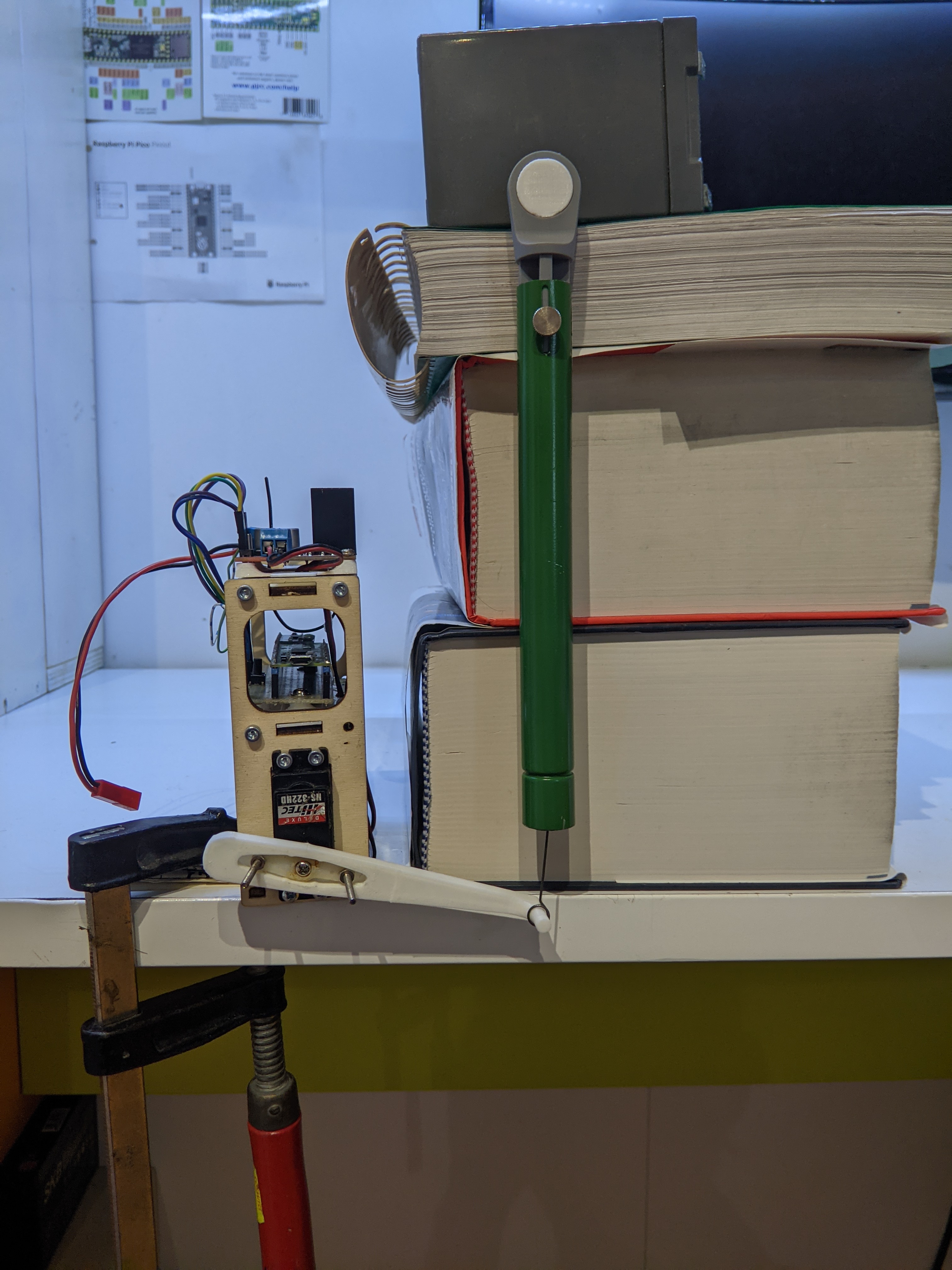
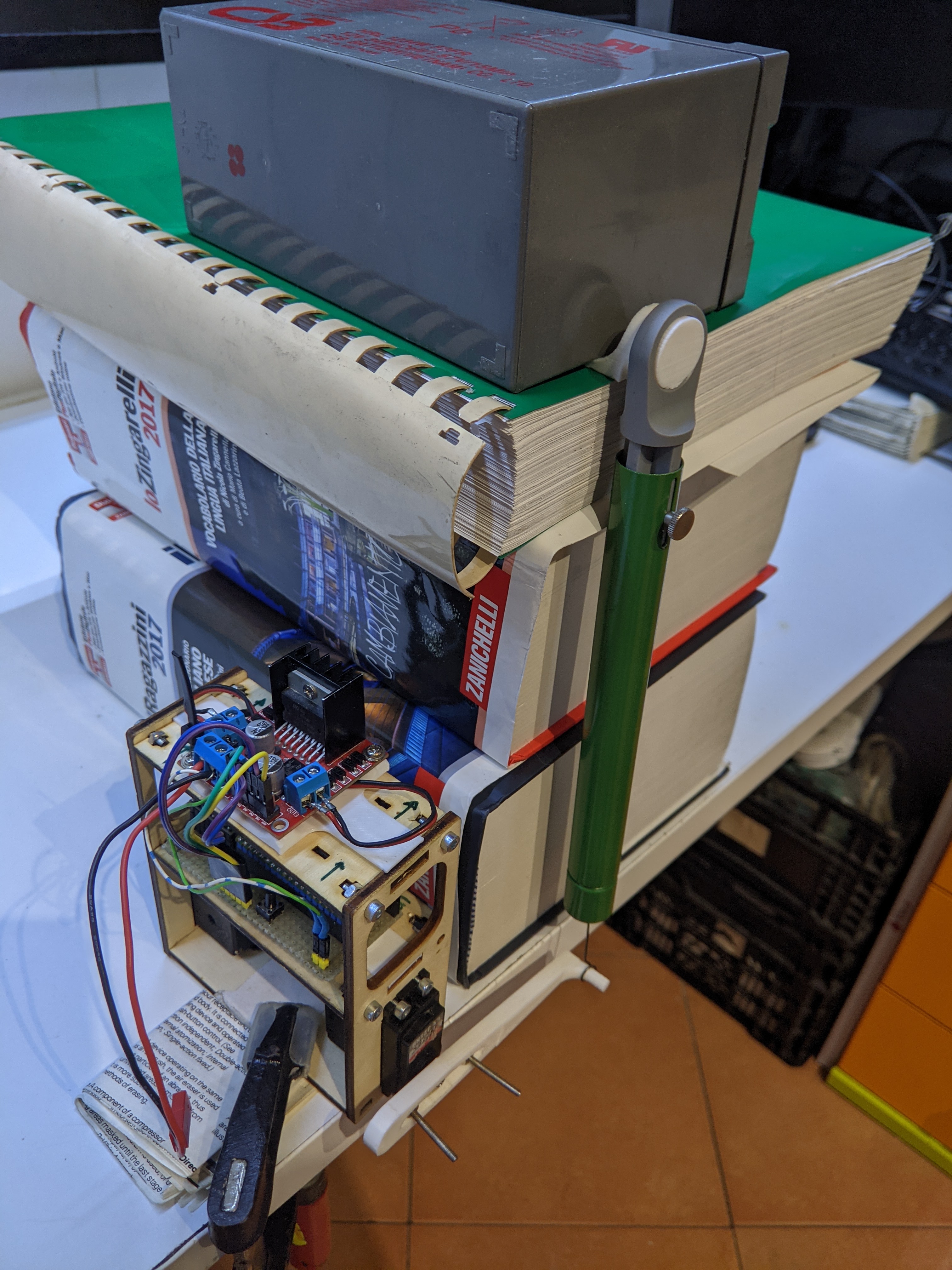
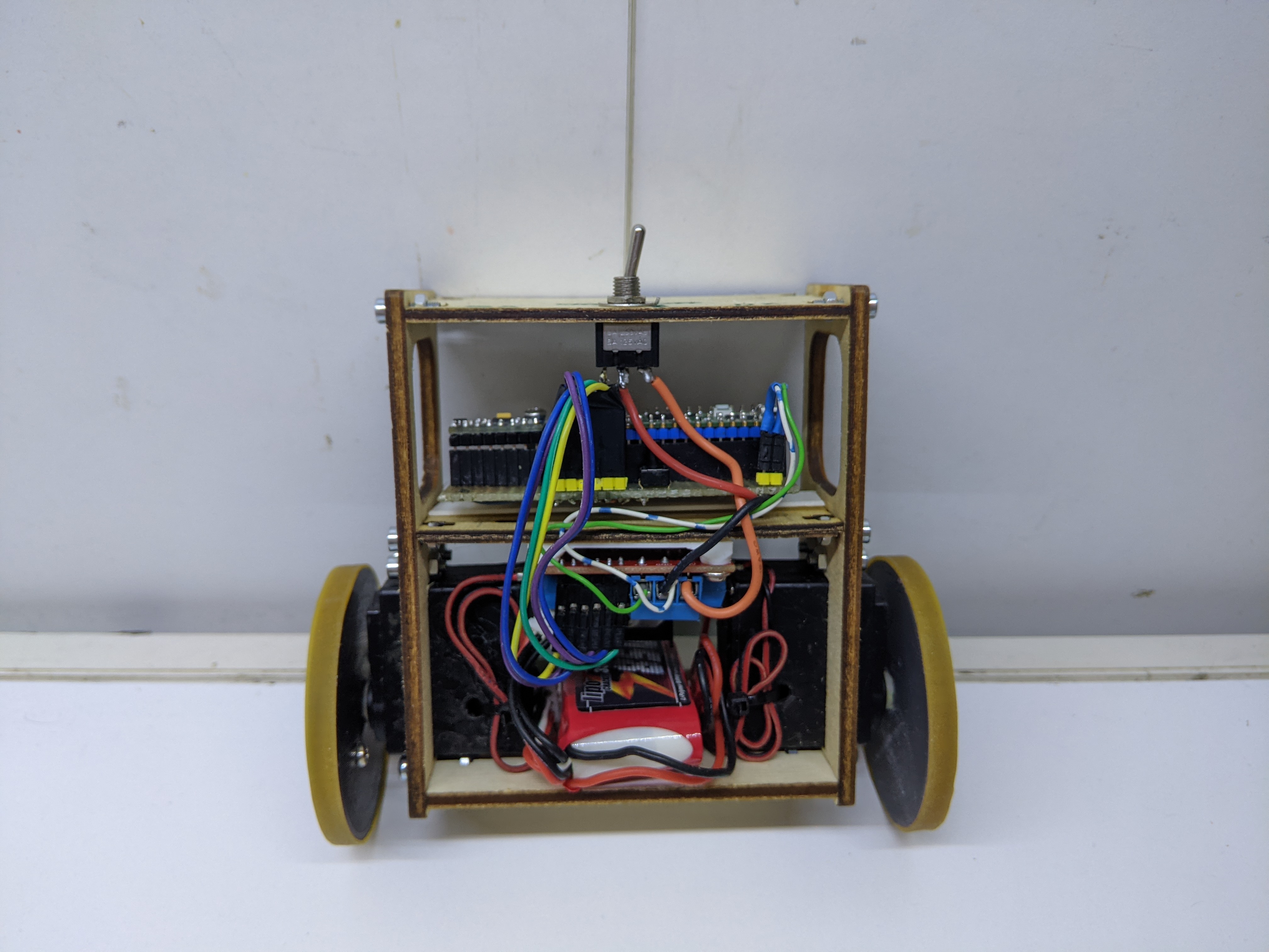
photos with the parts
The laser cut parts have some holes to be assembled into a 3d-dimensional shape. They also have some recesses to hold the 3d-printed parts onto which the electronics is mounted.
For the electronics, I decided to use a L298N motor driver I had laying around, Hitec HS-322D motors which we will talk more about in a sec, a RPi Pico as a microcontroller and a MPU6050 IMU to read the pitch angle $\theta$.
For the software, I used the Arduino-Pico framework to program the Pico with the Arduino framework, which gave me the possibility to use the ArduPID library, which I had used in the past to implement PID controllers, and the FastIMU library to read the IMU.
Now IMUs are an interesting piece of tech. The MPU6050 in particular is a 6-axis IMU which packs a 3 (cartesian) axis accelerometer and a 3 (rotational) axis gyroscope. The former measured the linear acceleration along each axis, the latter measures the angular velocity with which the IMU is rotating along a given cartesian axis. Neither of them are really usable on their own: accelerometers are really noisy sensors and they can only be used to to determine roll (around x axis) and pitch (around y axis) angles; gyroscopes on the other hand seem more fit for the job: it seems like we could just integrate velocity over time to obtain an angular position. That is true, but unfortunately for us gyroscopes have an intrisic bias, which when integrated over time tends to make the error between the measured angular position and the real one diverge.
Data obtained from accelerometers and gyroscopes can however be mixed together to obtain new, more reliable data. This technique is called sensor fusion. In general we are trying to do attitude estimation, though we are only really interested in the pitch angle for now. The most basic implementazion is a simple complementary filter, but that worked really poorly (you can still see my code in the repo). Ideally, one should implement a Kalman filter. I decided against that because I simply did not have the time to learn about them. I then decided to settle on a Madgwick filter (another interesting read), which was provided by the FastIMU library. The Madgwick filter is actually more of an algorithm to perform sensor fusion on IMU data. Internally it uses a Kalman filter, but also has a gradient descent step to reach minimum error.
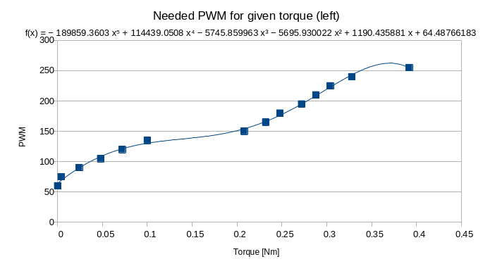
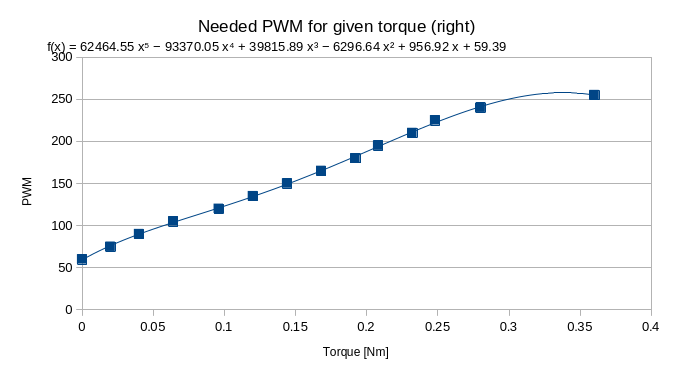
Finally, the motors. In a DC motor (even a DC gearmotor like the ones I am using) exerted torque is linearly proportional to the current flowing in the motor windings. Usually this linear relationship is provided by the motor datasheet. My motors, however, lacked such information. How fun. So I decided to derive myself a relation ship between the PWM value applied to the motors and the exerted torque. I 3d-printed a little arm to connect the motor and a dynamometer. I then measured the force reported by the dynamometer at different PWM levels and put in libreoffice calc to graph the curve of pwm against torque (torque is equal to force multiplied by the arm’s length). I then had libreoffice fit a 5th order polynomial to the curve, to finally obtain a relationship between the desired torque and the PWM required to obtain it.
Ok everything is working, time to test!
Ok, it sucks. But why is that? As I may have hinted at before, these motors suck. Hard. While they do exert the torque they advertise (and I measured that!) they to have a terrible deadzone. A deadzone is the set of inputs for which the output stays 0 even if in theory we should expect it to be different than zero. These motors have a HUGE deadzone. They do not start spinning until almost at half of the max PWM. This makes accurately controlling torque pratically impossible. From the video you can clearly see and ear that the motors are always running at max PWM. In this condition it’s almost like doing bang-bang control.
Furthermore, these two motors, which should be pretty similar to one another, actually are pretty different and tend to spind at different speeds for the same torque. That’s why the robot starts turning on itself. This is also a limitation of the mathematical model we used: we assumed the robot only had one wheel, actuated by one motor, and therefore we have no way of studying and controlling how the robot turns on itself.
This movement causes the robot to turn by almost 90 degrees. My desk is slightly tilted (measured it with a level). The desk being tilted is a disturbance for the system, and the robot needs to perpetually move forward to counter the disturbance and keep upright. The motors however cannot keep up with such a small disturbance and immediately saturate without being able to apply enough torque to rebalance the robot, and so it falls.
All this problems can be solved buy getting better motors. For the v2, I decided to try and use stepper motors, which are controlled in angular position and not in torque. Here a sneaky preview of how that turned out.
References
- P. Frankovský and L. Dominik and A. Gmiterko and I. Virgala: “Modeling of two-wheeled self-balancing robot driven by DC gearmotors”
- Felix Grasser and Aldo D’Arrigo and Silvio Colombi and Alfred C. Rufer: “JOE: A Mobile, Inverted Pendulum”